Parsing Histograms
This page demonstrates the parsing process for histogram events.
Preparing Sample Event Logs
First, let’s import some libraries and prepare the environment for our sample event logs:
>>> import os
>>> import tempfile
>>> import numpy as np
>>> # Define some constants
>>> RND_STATE = 1234
>>> N_EVENTS = 10
>>> N_PARTICLES = 1000
>>> MU = 0
>>> SIGMA = 2
>>> # Prepare temp dirs for storing event files
>>> tmpdirs = {}
Before parsing a event file, we need to generate it first. The sample event files are generated by three commonly used event log writers.
We can generate the events by PyTorch:
>>> tmpdirs['torch'] = tempfile.TemporaryDirectory()
>>> from torch.utils.tensorboard import SummaryWriter
>>> log_dir = tmpdirs['torch'].name
>>> writer = SummaryWriter(log_dir)
>>> rng = np.random.RandomState(RND_STATE)
>>> for i in range(N_EVENTS):
...   x = rng.normal(MU, SIGMA, size=N_PARTICLES)
...   writer.add_histogram('dist', x + i, i)
>>> writer.close()
and quickly check the results:
>>> from tbparse import SummaryReader
>>> SummaryReader(log_dir, pivot=True).histograms.columns
Index(['step', 'dist/counts', 'dist/limits'], dtype='object')
We can generate the events by TensorFlow2 / Keras:
>>> tmpdirs['tensorflow'] = tempfile.TemporaryDirectory()
>>> import tensorflow as tf
>>> log_dir = tmpdirs['tensorflow'].name
>>> writer = tf.summary.create_file_writer(log_dir)
>>> writer.set_as_default()
>>> rng = np.random.RandomState(RND_STATE)
>>> for i in range(N_EVENTS):
...   x = rng.normal(MU, SIGMA, size=N_PARTICLES)
...   assert tf.summary.histogram('dist', x + i, i)
>>> writer.close()
and quickly check the results:
>>> from tbparse import SummaryReader
>>> SummaryReader(log_dir, pivot=True).tensors.columns
Index(['step', 'dist'], dtype='object')
Warning
In the new versions of TensorFlow, the histogram method actually
stores the events as tensors events inside the event file. Thus, you should perform
an extra step with tensor_to_histogram() beforehand
if the event file is generated by TensorFlow2. (An example is shown later)
We can generate the events by TensorboardX:
>>> tmpdirs['tensorboardX'] = tempfile.TemporaryDirectory()
>>> from tensorboardX import SummaryWriter
>>> log_dir = tmpdirs['tensorboardX'].name
>>> writer = SummaryWriter(log_dir)
>>> rng = np.random.RandomState(RND_STATE)
>>> for i in range(N_EVENTS):
...   x = rng.normal(MU, SIGMA, size=N_PARTICLES)
...   writer.add_histogram('dist', x + i, i)
>>> writer.close()
and quickly check the results:
>>> from tbparse import SummaryReader
>>> SummaryReader(log_dir, pivot=True).histograms.columns
Index(['step', 'dist/counts', 'dist/limits'], dtype='object')
The event logs can be easily read in 2 lines of code as shown above (1 for importing tbparse, 1 for reading the events).
Parsing Event Logs
In different use cases, we will want to read the event logs in different styles.
We further show different configurations of the tbparse.SummaryReader class.
Load Event File / Run Directory
>>> from tbparse import SummaryReader
>>> log_dir = tmpdirs['torch'].name
>>> # Long Format
>>> df = SummaryReader(log_dir).histograms
>>> df.columns
Index(['step', 'tag', 'counts', 'limits'], dtype='object')
>>> # Wide Format
>>> df = SummaryReader(log_dir, pivot=True).histograms
>>> df.columns
Index(['step', 'dist/counts', 'dist/limits'], dtype='object')
>>> from tbparse import SummaryReader
>>> log_dir = tmpdirs['tensorflow'].name
>>> # Long Format
>>> df = SummaryReader(log_dir).tensors
>>> df.columns
Index(['step', 'tag', 'value'], dtype='object')
>>> hist_dict_arr = df['value'].apply(SummaryReader.tensor_to_histogram)
>>> df['counts'] = hist_dict_arr.apply(lambda x: x['counts'])
>>> df['limits'] = hist_dict_arr.apply(lambda x: x['limits'])
>>> df.drop(columns=['value'], inplace=True)
>>> df.columns
Index(['step', 'tag', 'counts', 'limits'], dtype='object')
>>> # Wide Format
>>> df = SummaryReader(log_dir, pivot=True).tensors
>>> df.columns
Index(['step', 'dist'], dtype='object')
>>> hist_dict_arr = df['dist'].apply(SummaryReader.tensor_to_histogram)
>>> df['dist/counts'] = hist_dict_arr.apply(lambda x: x['counts'])
>>> df['dist/limits'] = hist_dict_arr.apply(lambda x: x['limits'])
>>> df.drop(columns=['dist'], inplace=True)
>>> df.columns
Index(['step', 'dist/counts', 'dist/limits'], dtype='object')
>>> from tbparse import SummaryReader
>>> log_dir = tmpdirs['tensorboardX'].name
>>> # Long Format
>>> df = SummaryReader(log_dir).histograms
>>> df.columns
Index(['step', 'tag', 'counts', 'limits'], dtype='object')
>>> # Wide Format
>>> df = SummaryReader(log_dir, pivot=True).histograms
>>> df.columns
Index(['step', 'dist/counts', 'dist/limits'], dtype='object')
Warning
When accessing SummaryReader.histograms, the events stored in
each event file are collected internally. The best practice is to store the
returned results in a DataFrame as shown in the samples, instead of repeatedly
accessing SummaryReader.histograms.
Extra Columns
See the Extra Columns page for more details.
Plotting Events
We further demonstrate some basic filtering techniques for plotting our data.
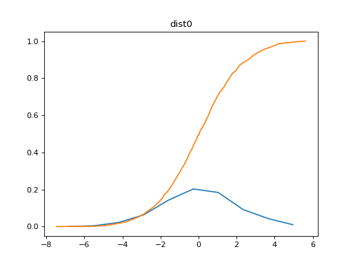
Plotting a Distribution
The data from tensorboard event logs:
import matplotlib.pyplot as plt
from tbparse import SummaryReader

log_dir = tmpdirs['torch'].name
reader = SummaryReader(log_dir, pivot=True)
df = reader.histograms
df.set_index('step', inplace=True)
counts0 = df.at[0, 'dist/counts']
limits0 = df.at[0, 'dist/limits']
# draw PDF
x = np.linspace(limits0[0], limits0[-1], 11)
x, y = SummaryReader.histogram_to_pdf(counts0, limits0, x)
plt.plot(x, y)
# draw CDF
x = np.linspace(limits0[0], limits0[-1], 1000)
y = SummaryReader.histogram_to_cdf(counts0, limits0, x)
plt.plot(x, y)
plt.title('dist0')
plt.show()
The data from tensorboard event logs:
import matplotlib.pyplot as plt
from tbparse import SummaryReader

log_dir = tmpdirs['tensorflow'].name
reader = SummaryReader(log_dir, pivot=True)
df = reader.tensors
buckets0 = df.at[0, 'dist']
hist_dict0 = SummaryReader.tensor_to_histogram(buckets0)
counts0 = hist_dict0['counts']
limits0 = hist_dict0['limits']
# draw PDF
x = np.linspace(limits0[0], limits0[-1], 11)
x, y = SummaryReader.histogram_to_pdf(counts0, limits0, x)
plt.plot(x, y)
# draw CDF
x = np.linspace(limits0[0], limits0[-1], 1000)
y = SummaryReader.histogram_to_cdf(counts0, limits0, x)
plt.plot(x, y)
plt.title('dist0')
plt.show()

The data from tensorboard event logs:
import matplotlib.pyplot as plt
from tbparse import SummaryReader

log_dir = tmpdirs['tensorboardX'].name
reader = SummaryReader(log_dir, pivot=True)
df = reader.histograms
df.set_index('step', inplace=True)
counts0 = df.at[0, 'dist/counts']
limits0 = df.at[0, 'dist/limits']
# draw PDF
x = np.linspace(limits0[0], limits0[-1], 11)
x, y = SummaryReader.histogram_to_pdf(counts0, limits0, x)
plt.plot(x, y)
# draw CDF
x = np.linspace(limits0[0], limits0[-1], 1000)
y = SummaryReader.histogram_to_cdf(counts0, limits0, x)
plt.plot(x, y)
plt.title('dist0')
plt.show()

The ground truth data:
import scipy.stats
import matplotlib.pyplot as plt
from tbparse import SummaryReader

rng = np.random.RandomState(RND_STATE)
x = rng.normal(MU, SIGMA, size=N_PARTICLES)
counts, limits = np.histogram(x)
hist = (counts, limits)
hist_dist = scipy.stats.rv_histogram(hist)
centers = (limits[1:]+limits[:-1])/2
pdf = hist_dist.pdf(centers)
cdf = hist_dist.cdf(centers)
plt.plot(centers, pdf)
plt.plot(centers, cdf)
plt.hist(x, density=True)
plt.title('dist0')
plt.show()
Reference: https://docs.scipy.org/doc/scipy/reference/generated/scipy.stats.rv_histogram.html
Plotting Multiple (Stacked) Distributions
import seaborn as sns
import matplotlib.pyplot as plt
log_dir = tmpdirs['torch'].name
reader = SummaryReader(log_dir, pivot=True)
df = reader.histograms
# Set background
sns.set_theme(style="white", rc={"axes.facecolor": (0, 0, 0, 0)})
# Choose color palettes for the distributions
pal = sns.color_palette("Oranges", 20)[5:-5]
# Initialize the FacetGrid object (stacking multiple plots)
g = sns.FacetGrid(df, row='step', hue='step', aspect=15, height=.4, palette=pal)

def plot_subplots(x, color, label, data):
  ax = plt.gca()
  ax.text(0, .08, label, fontweight="bold", color=color,
          ha="left", va="center", transform=ax.transAxes)
  counts = data['dist/counts'].iloc[0]
  limits = data['dist/limits'].iloc[0]
  x = np.linspace(limits[0], limits[-1], 15)
  x, y = SummaryReader.histogram_to_pdf(counts, limits, x)
  # Draw the densities in a few steps
  sns.lineplot(x=x, y=y, clip_on=False, color="w", lw=2)
  ax.fill_between(x, y, color=color)
# Plot each subplots with df[df['step']==i]
g.map_dataframe(plot_subplots, None)

# Add a bottom line for each subplot
# passing color=None to refline() uses the hue mapping
g.refline(y=0, linewidth=2, linestyle="-", color=None, clip_on=False)
# Set the subplots to overlap (i.e., height of each distribution)
g.figure.subplots_adjust(hspace=-.9)
# Remove axes details that don't play well with overlap
g.set_titles("")
g.set(yticks=[], xlabel="", ylabel="")
g.despine(bottom=True, left=True)

import seaborn as sns
import matplotlib.pyplot as plt
log_dir = tmpdirs['tensorflow'].name
reader = SummaryReader(log_dir, pivot=True)
df = reader.tensors
# Set background
sns.set_theme(style="white", rc={"axes.facecolor": (0, 0, 0, 0)})
# Choose color palettes for the distributions
pal = sns.color_palette("Oranges", 20)[5:-5]
# Initialize the FacetGrid object (stacking multiple plots)
g = sns.FacetGrid(df, row='step', hue='step', aspect=15, height=.4, palette=pal)

def plot_subplots(x, color, label, data):
  ax = plt.gca()
  ax.text(0, .08, label, fontweight="bold", color=color,
          ha="left", va="center", transform=ax.transAxes)
  buckets = data['dist'].iloc[0]
  hist_dict = SummaryReader.tensor_to_histogram(buckets)
  counts = hist_dict['counts']
  limits = hist_dict['limits']
  x = np.linspace(limits[0], limits[-1], 15)
  x, y = SummaryReader.histogram_to_pdf(counts, limits, x)
  # Draw the densities in a few steps
  sns.lineplot(x=x, y=y, clip_on=False, color="w", lw=2)
  ax.fill_between(x, y, color=color)
# Plot each subplots with df[df['step']==i]
g.map_dataframe(plot_subplots, None)

# Add a bottom line for each subplot
# passing color=None to refline() uses the hue mapping
g.refline(y=0, linewidth=2, linestyle="-", color=None, clip_on=False)
# Set the subplots to overlap
# Set the subplots to overlap (i.e., height of each distribution)
g.figure.subplots_adjust(hspace=-.9)
# Remove axes details that don't play well with overlap
g.set_titles("")
g.set(yticks=[], xlabel="", ylabel="")
g.despine(bottom=True, left=True)

import seaborn as sns
import matplotlib.pyplot as plt
log_dir = tmpdirs['tensorboardX'].name
reader = SummaryReader(log_dir, pivot=True)
df = reader.histograms
# Set background
sns.set_theme(style="white", rc={"axes.facecolor": (0, 0, 0, 0)})
# Choose color palettes for the distributions
pal = sns.color_palette("Oranges", 20)[5:-5]
# Initialize the FacetGrid object (stacking multiple plots)
g = sns.FacetGrid(df, row='step', hue='step', aspect=15, height=.4, palette=pal)

def plot_subplots(x, color, label, data):
  ax = plt.gca()
  ax.text(0, .08, label, fontweight="bold", color=color,
          ha="left", va="center", transform=ax.transAxes)
  counts = data['dist/counts'].iloc[0]
  limits = data['dist/limits'].iloc[0]
  x = np.linspace(limits[0], limits[-1], 15)
  x, y = SummaryReader.histogram_to_pdf(counts, limits, x)
  # Draw the densities in a few steps
  sns.lineplot(x=x, y=y, clip_on=False, color="w", lw=2)
  ax.fill_between(x, y, color=color)
# Plot each subplots with df[df['step']==i]
g.map_dataframe(plot_subplots, None)

# Add a bottom line for each subplot
# passing color=None to refline() uses the hue mapping
g.refline(y=0, linewidth=2, linestyle="-", color=None, clip_on=False)
# Set the subplots to overlap (i.e., height of each distribution)
g.figure.subplots_adjust(hspace=-.9)
# Remove axes details that don't play well with overlap
g.set_titles("")
g.set(yticks=[], xlabel="", ylabel="")
g.despine(bottom=True, left=True)
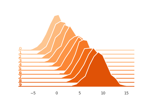
Reference: https://seaborn.pydata.org/examples/kde_ridgeplot.html
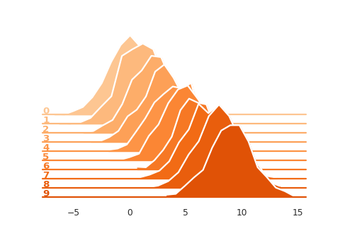
Plotting Multiple (Stacked) Histograms
import seaborn as sns
import matplotlib.pyplot as plt
log_dir = tmpdirs['torch'].name
reader = SummaryReader(log_dir, pivot=True)
df = reader.histograms
# Set background
sns.set_theme(style="white", rc={"axes.facecolor": (0, 0, 0, 0)})
# Choose color palettes for the distributions
pal = sns.color_palette("Oranges", 20)[5:-5]
# Initialize the FacetGrid object (stacking multiple plots)
g = sns.FacetGrid(df, row='step', hue='step', aspect=15, height=.4, palette=pal)

def plot_subplots(x, color, label, data):
  ax = plt.gca()
  ax.text(0, .08, label, fontweight="bold", color=color,
          ha="left", va="center", transform=ax.transAxes)
  counts = data['dist/counts'].iloc[0]
  limits = data['dist/limits'].iloc[0]
  x, y = SummaryReader.histogram_to_bins(counts, limits, limits[0], limits[-1], 15)
  # Draw the densities in a few steps
  sns.lineplot(x=x, y=y, clip_on=False, color="w", lw=2)
  ax.fill_between(x, y, color=color)
# Plot each subplots with df[df['step']==i]
g.map_dataframe(plot_subplots, None)

# Add a bottom line for each subplot
# passing color=None to refline() uses the hue mapping
g.refline(y=0, linewidth=2, linestyle="-", color=None, clip_on=False)
# Set the subplots to overlap (i.e., height of each distribution)
g.figure.subplots_adjust(hspace=-.9)
# Remove axes details that don't play well with overlap
g.set_titles("")
g.set(yticks=[], xlabel="", ylabel="")
g.despine(bottom=True, left=True)

import seaborn as sns
import matplotlib.pyplot as plt
log_dir = tmpdirs['tensorflow'].name
reader = SummaryReader(log_dir, pivot=True)
df = reader.tensors
# Set background
sns.set_theme(style="white", rc={"axes.facecolor": (0, 0, 0, 0)})
# Choose color palettes for the distributions
pal = sns.color_palette("Oranges", 20)[5:-5]
# Initialize the FacetGrid object (stacking multiple plots)
g = sns.FacetGrid(df, row='step', hue='step', aspect=15, height=.4, palette=pal)

def plot_subplots(x, color, label, data):
  ax = plt.gca()
  ax.text(0, .08, label, fontweight="bold", color=color,
          ha="left", va="center", transform=ax.transAxes)
  buckets = data['dist'].iloc[0]
  hist_dict = SummaryReader.tensor_to_histogram(buckets)
  counts = hist_dict['counts']
  limits = hist_dict['limits']
  x, y = SummaryReader.histogram_to_bins(counts, limits, limits[0], limits[-1], 15)
  # Draw the densities in a few steps
  sns.lineplot(x=x, y=y, clip_on=False, color="w", lw=2)
  ax.fill_between(x, y, color=color)
# Plot each subplots with df[df['step']==i]
g.map_dataframe(plot_subplots, None)

# Add a bottom line for each subplot
# passing color=None to refline() uses the hue mapping
g.refline(y=0, linewidth=2, linestyle="-", color=None, clip_on=False)
# Set the subplots to overlap
# Set the subplots to overlap (i.e., height of each distribution)
g.figure.subplots_adjust(hspace=-.9)
# Remove axes details that don't play well with overlap
g.set_titles("")
g.set(yticks=[], xlabel="", ylabel="")
g.despine(bottom=True, left=True)
import seaborn as sns
import matplotlib.pyplot as plt
log_dir = tmpdirs['tensorboardX'].name
reader = SummaryReader(log_dir, pivot=True)
df = reader.histograms
# Set background
sns.set_theme(style="white", rc={"axes.facecolor": (0, 0, 0, 0)})
# Choose color palettes for the distributions
pal = sns.color_palette("Oranges", 20)[5:-5]
# Initialize the FacetGrid object (stacking multiple plots)
g = sns.FacetGrid(df, row='step', hue='step', aspect=15, height=.4, palette=pal)

def plot_subplots(x, color, label, data):
  ax = plt.gca()
  ax.text(0, .08, label, fontweight="bold", color=color,
          ha="left", va="center", transform=ax.transAxes)
  counts = data['dist/counts'].iloc[0]
  limits = data['dist/limits'].iloc[0]
  x, y = SummaryReader.histogram_to_bins(counts, limits, limits[0], limits[-1], 15)
  # Draw the densities in a few steps
  sns.lineplot(x=x, y=y, clip_on=False, color="w", lw=2)
  ax.fill_between(x, y, color=color)
# Plot each subplots with df[df['step']==i]
g.map_dataframe(plot_subplots, None)

# Add a bottom line for each subplot
# passing color=None to refline() uses the hue mapping
g.refline(y=0, linewidth=2, linestyle="-", color=None, clip_on=False)
# Set the subplots to overlap (i.e., height of each distribution)
g.figure.subplots_adjust(hspace=-.9)
# Remove axes details that don't play well with overlap
g.set_titles("")
g.set(yticks=[], xlabel="", ylabel="")
g.despine(bottom=True, left=True)
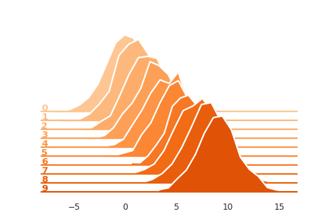
SummaryReader.histogram_to_bins aims to reproduce the visualization in
tensorboard dashboard.