Parsing Scalars
This page demonstrates the parsing process for scalar events.
Preparing Sample Event Logs
First, let’s import some libraries and prepare the environment for our sample event logs:
>>> import os
>>> import tempfile
>>> # Define some constants
>>> N_RUNS = 2
>>> N_EVENTS = 3
>>> # Prepare temp dirs for storing event files
>>> tmpdirs = {}
Before parsing a event file, we need to generate it first. The sample event files are generated by three commonly used event log writers.
We can generate the events by PyTorch:
>>> tmpdirs['torch'] = tempfile.TemporaryDirectory()
>>> from torch.utils.tensorboard import SummaryWriter
>>> log_dir = tmpdirs['torch'].name
>>> for i in range(N_RUNS): # 2 independent runs
...   writer = SummaryWriter(os.path.join(log_dir, f'run{i}'))
...   for j in range(N_EVENTS): # stores 2 tags, each with 3 events
...     writer.add_scalar('y=2x+C', j * 2 + i, j)
...     writer.add_scalar('y=3x+C', j * 3 + i, j)
...   writer.close()
and quickly check the results:
>>> from tbparse import SummaryReader
>>> SummaryReader(log_dir, pivot=True).scalars
   step      y=2x+C      y=3x+C
0     0  [0.0, 1.0]  [0.0, 1.0]
1     1  [2.0, 3.0]  [3.0, 4.0]
2     2  [4.0, 5.0]  [6.0, 7.0]
We can generate the events by TensorFlow2 / Keras:
>>> tmpdirs['tensorflow'] = tempfile.TemporaryDirectory()
>>> import tensorflow as tf
>>> log_dir = tmpdirs['tensorflow'].name
>>> for i in range(N_RUNS): # 2 independent runs
...   writer = tf.summary.create_file_writer(os.path.join(log_dir, f'run{i}'))
...   writer.set_as_default()
...   for j in range(N_EVENTS): # stores 2 tags, each with 3 events
...     assert tf.summary.scalar('y=2x+C', j * 2 + i, j)
...     assert tf.summary.scalar('y=3x+C', j * 3 + i, j)
...   writer.close()
and quickly check the results:
>>> from tbparse import SummaryReader
>>> SummaryReader(log_dir, pivot=True).scalars
Empty DataFrame
Columns: []
Index: []
Warning
In the new versions of TensorFlow, the scalar method actually
stores the events as tensors events inside the event file. Thus, you should refer to
the Parsing Tensors page if the event file is generated by TensorFlow2.
We can generate the events by TensorboardX:
>>> tmpdirs['tensorboardX'] = tempfile.TemporaryDirectory()
>>> from tensorboardX import SummaryWriter
>>> log_dir = tmpdirs['tensorboardX'].name
>>> for i in range(N_RUNS): # 2 independent runs
...   writer = SummaryWriter(os.path.join(log_dir, f'run{i}'))
...   for j in range(N_EVENTS): # stores 2 tags, each with 3 events
...     writer.add_scalar('y=2x+C', j * 2 + i, j)
...     writer.add_scalar('y=3x+C', j * 3 + i, j)
...   writer.close()
and quickly check the results:
>>> from tbparse import SummaryReader
>>> SummaryReader(log_dir, pivot=True).scalars
   step      y_2x_C      y_3x_C
0     0  [0.0, 1.0]  [0.0, 1.0]
1     1  [2.0, 3.0]  [3.0, 4.0]
2     2  [4.0, 5.0]  [6.0, 7.0]
Warning
TensorboardX automatically escapes special character
=, + in the tags.
The event logs can be easily read in 2 lines of code as shown above (1 for importing tbparse, 1 for reading the events).
Parsing Event Logs
In different use cases, we will want to read the event logs in different styles.
We further show different configurations of the tbparse.SummaryReader class.
Load Event File
We can load a single event file with its file path:
We first store the file path in the event_file variable.
>>> log_dir = tmpdirs['torch'].name
>>> run_dir = os.path.join(log_dir, 'run0')
>>> event_file = os.path.join(run_dir, sorted(os.listdir(run_dir))[0])
The pivot parameter in SummaryReader determines the event format:
If
pivot=False(default), the events are stored in Long format.If
pivot=True, the events are stored in Wide format.
>>> from tbparse import SummaryReader
>>> reader = SummaryReader(event_file) # long format
>>> df = reader.scalars
>>> df
   step     tag  value
0     0  y=2x+C    0.0
1     1  y=2x+C    2.0
2     2  y=2x+C    4.0
3     0  y=3x+C    0.0
4     1  y=3x+C    3.0
5     2  y=3x+C    6.0
>>> df[df['tag'] == 'y=2x+C'] # filter out 'y=3x+C'
   step     tag  value
0     0  y=2x+C    0.0
1     1  y=2x+C    2.0
2     2  y=2x+C    4.0
>>> df[df['tag'] == 'y=2x+C']['value'] # as pandas.Series
0    0.0
1    2.0
2    4.0
Name: value, dtype: float64
>>> df[df['tag'] == 'y=2x+C']['value'].to_numpy() # as numpy array
array([0., 2., 4.])
>>> df[df['tag'] == 'y=2x+C']['value'].to_list() # as list
[0.0, 2.0, 4.0]
>>> from tbparse import SummaryReader
>>> reader = SummaryReader(event_file, pivot=True) # wide format
>>> df = reader.scalars
>>> df
   step  y=2x+C  y=3x+C
0     0     0.0     0.0
1     1     2.0     3.0
2     2     4.0     6.0
>>> df[['step', 'y=2x+C']] # filter out 'y=3x+C'
   step  y=2x+C
0     0     0.0
1     1     2.0
2     2     4.0
>>> df['y=2x+C'] # as pandas.Series
0    0.0
1    2.0
2    4.0
Name: y=2x+C, dtype: float64
>>> df['y=2x+C'].to_numpy() # as numpy array
array([0., 2., 4.])
>>> df['y=2x+C'].to_list() # as list
[0.0, 2.0, 4.0]
We first store the file path in the event_file variable.
>>> log_dir = tmpdirs['tensorboardX'].name
>>> run_dir = os.path.join(log_dir, 'run0')
>>> event_file = os.path.join(run_dir, sorted(os.listdir(run_dir))[0])
The pivot parameter in SummaryReader determines the event format:
If
pivot=False(default), the events are stored in Long format.If
pivot=True, the events are stored in Wide format.
>>> from tbparse import SummaryReader
>>> reader = SummaryReader(event_file) # long format
>>> df = reader.scalars
>>> df
   step     tag  value
0     0  y_2x_C    0.0
1     1  y_2x_C    2.0
2     2  y_2x_C    4.0
3     0  y_3x_C    0.0
4     1  y_3x_C    3.0
5     2  y_3x_C    6.0
>>> df[df['tag'] == 'y_2x_C'] # filter out 'y_3x_C'
   step     tag  value
0     0  y_2x_C    0.0
1     1  y_2x_C    2.0
2     2  y_2x_C    4.0
>>> df[df['tag'] == 'y_2x_C']['value'] # as pandas.Series
0    0.0
1    2.0
2    4.0
Name: value, dtype: float64
>>> df[df['tag'] == 'y_2x_C']['value'].to_numpy() # as numpy array
array([0., 2., 4.])
>>> df[df['tag'] == 'y_2x_C']['value'].to_list() # as list
[0.0, 2.0, 4.0]
>>> from tbparse import SummaryReader
>>> reader = SummaryReader(event_file, pivot=True) # wide format
>>> df = reader.scalars
>>> df
   step  y_2x_C  y_3x_C
0     0     0.0     0.0
1     1     2.0     3.0
2     2     4.0     6.0
>>> df[['step', 'y_2x_C']] # filter out 'y_3x_C'
   step  y_2x_C
0     0     0.0
1     1     2.0
2     2     4.0
>>> df['y_2x_C'] # as pandas.Series
0    0.0
1    2.0
2    4.0
Name: y_2x_C, dtype: float64
>>> df['y_2x_C'].to_numpy() # as numpy array
array([0., 2., 4.])
>>> df['y_2x_C'].to_list() # as list
[0.0, 2.0, 4.0]
Load Run Directory
We can load all event files under a directory (an experiment run):
We first store the run directory path in the run_dir variable.
>>> log_dir = tmpdirs['torch'].name
>>> run_dir = os.path.join(log_dir, 'run0')
The pivot parameter in SummaryReader determines the event format:
>>> reader = SummaryReader(run_dir)
>>> reader.scalars
   step     tag  value
0     0  y=2x+C    0.0
1     1  y=2x+C    2.0
2     2  y=2x+C    4.0
3     0  y=3x+C    0.0
4     1  y=3x+C    3.0
5     2  y=3x+C    6.0
>>> reader = SummaryReader(run_dir, pivot=True)
>>> reader.scalars
   step  y=2x+C  y=3x+C
0     0     0.0     0.0
1     1     2.0     3.0
2     2     4.0     6.0
We first store the run directory path in the run_dir variable.
>>> log_dir = tmpdirs['tensorboardX'].name
>>> run_dir = os.path.join(log_dir, 'run0')
The pivot parameter in SummaryReader determines the event format:
>>> reader = SummaryReader(run_dir)
>>> reader.scalars
   step     tag  value
0     0  y_2x_C    0.0
1     1  y_2x_C    2.0
2     2  y_2x_C    4.0
3     0  y_3x_C    0.0
4     1  y_3x_C    3.0
5     2  y_3x_C    6.0
>>> reader = SummaryReader(run_dir, pivot=True)
>>> reader.scalars
   step  y_2x_C  y_3x_C
0     0     0.0     0.0
1     1     2.0     3.0
2     2     4.0     6.0
If your run directory contains multiple event files, SummaryReader
will collect all events stored inside them into the DataFrame.
(The sample result here stays the same since we do not have
multiple event files stored in our sample run directory.)
Load Log Directory
We can further load all runs under the log directory.
We first store the log directory path in the log_dir variable.
>>> log_dir = tmpdirs['torch'].name
The pivot parameter in SummaryReader determines the event format.
The extra_columns parameter in SummaryReader determines
the extra columns to be stored in the DataFrame:
>>> reader = SummaryReader(log_dir)
>>> reader.scalars
    step     tag  value
0      0  y=2x+C    0.0
1      0  y=2x+C    1.0
2      1  y=2x+C    2.0
3      1  y=2x+C    3.0
4      2  y=2x+C    4.0
5      2  y=2x+C    5.0
6      0  y=3x+C    0.0
7      0  y=3x+C    1.0
8      1  y=3x+C    3.0
9      1  y=3x+C    4.0
10     2  y=3x+C    6.0
11     2  y=3x+C    7.0
>>> reader = SummaryReader(log_dir, extra_columns={'dir_name'}) # with event directory name
>>> reader.scalars
    step     tag  value dir_name
0      0  y=2x+C    0.0     run0
1      1  y=2x+C    2.0     run0
2      2  y=2x+C    4.0     run0
3      0  y=3x+C    0.0     run0
4      1  y=3x+C    3.0     run0
5      2  y=3x+C    6.0     run0
6      0  y=2x+C    1.0     run1
7      1  y=2x+C    3.0     run1
8      2  y=2x+C    5.0     run1
9      0  y=3x+C    1.0     run1
10     1  y=3x+C    4.0     run1
11     2  y=3x+C    7.0     run1
>>> df = reader.scalars
>>> df[df['dir_name'] == 'run0'] # filter events in run0
   step     tag  value dir_name
0     0  y=2x+C    0.0     run0
1     1  y=2x+C    2.0     run0
2     2  y=2x+C    4.0     run0
3     0  y=3x+C    0.0     run0
4     1  y=3x+C    3.0     run0
5     2  y=3x+C    6.0     run0
>>> reader = SummaryReader(log_dir, pivot=True)
>>> reader.scalars
   step      y=2x+C      y=3x+C
0     0  [0.0, 1.0]  [0.0, 1.0]
1     1  [2.0, 3.0]  [3.0, 4.0]
2     2  [4.0, 5.0]  [6.0, 7.0]
>>> reader = SummaryReader(log_dir, pivot=True, extra_columns={'dir_name'}) # with event directory name
>>> reader.scalars
   step  y=2x+C  y=3x+C dir_name
0     0     0.0     0.0     run0
1     1     2.0     3.0     run0
2     2     4.0     6.0     run0
3     0     1.0     1.0     run1
4     1     3.0     4.0     run1
5     2     5.0     7.0     run1
>>> df = reader.scalars
>>> df[df['dir_name'] == 'run0'] # filter events in run0
   step  y=2x+C  y=3x+C dir_name
0     0     0.0     0.0     run0
1     1     2.0     3.0     run0
2     2     4.0     6.0     run0
We first store the log directory path in the log_dir variable.
>>> log_dir = tmpdirs['tensorboardX'].name
The pivot parameter in SummaryReader determines the event format.
The extra_columns parameter in SummaryReader determines
the extra columns to be stored in the DataFrame:
>>> reader = SummaryReader(log_dir)
>>> reader.scalars
    step     tag  value
0      0  y_2x_C    0.0
1      0  y_2x_C    1.0
2      1  y_2x_C    2.0
3      1  y_2x_C    3.0
4      2  y_2x_C    4.0
5      2  y_2x_C    5.0
6      0  y_3x_C    0.0
7      0  y_3x_C    1.0
8      1  y_3x_C    3.0
9      1  y_3x_C    4.0
10     2  y_3x_C    6.0
11     2  y_3x_C    7.0
>>> reader = SummaryReader(log_dir, extra_columns={'dir_name'}) # with event dir name
>>> reader.scalars
    step     tag  value dir_name
0      0  y_2x_C    0.0     run0
1      1  y_2x_C    2.0     run0
2      2  y_2x_C    4.0     run0
3      0  y_3x_C    0.0     run0
4      1  y_3x_C    3.0     run0
5      2  y_3x_C    6.0     run0
6      0  y_2x_C    1.0     run1
7      1  y_2x_C    3.0     run1
8      2  y_2x_C    5.0     run1
9      0  y_3x_C    1.0     run1
10     1  y_3x_C    4.0     run1
11     2  y_3x_C    7.0     run1
>>> df = reader.scalars
>>> df[df['dir_name'] == 'run0'] # filter events in run0
   step     tag  value dir_name
0     0  y_2x_C    0.0     run0
1     1  y_2x_C    2.0     run0
2     2  y_2x_C    4.0     run0
3     0  y_3x_C    0.0     run0
4     1  y_3x_C    3.0     run0
5     2  y_3x_C    6.0     run0
>>> reader = SummaryReader(log_dir, pivot=True)
>>> reader.scalars
   step      y_2x_C      y_3x_C
0     0  [0.0, 1.0]  [0.0, 1.0]
1     1  [2.0, 3.0]  [3.0, 4.0]
2     2  [4.0, 5.0]  [6.0, 7.0]
>>> reader = SummaryReader(log_dir, pivot=True, extra_columns={'dir_name'}) # with event dir name
>>> reader.scalars
   step  y_2x_C  y_3x_C dir_name
0     0     0.0     0.0     run0
1     1     2.0     3.0     run0
2     2     4.0     6.0     run0
3     0     1.0     1.0     run1
4     1     3.0     4.0     run1
5     2     5.0     7.0     run1
>>> df = reader.scalars
>>> df[df['dir_name'] == 'run0'] # filter events in run0
   step  y_2x_C  y_3x_C dir_name
0     0     0.0     0.0     run0
1     1     2.0     3.0     run0
2     2     4.0     6.0     run0
Warning
When accessing SummaryReader.scalars, the events stored in
each event file are collected internally. The best practice is to store the
returned results in a DataFrame as shown in the samples, instead of repeatedly
accessing SummaryReader.scalars.
Extra Columns
See the Extra Columns page for more details.
Plotting Events
We recommend using seaborn for most plotting, since its API is both
flexible and friendly. When you need to tweak some details of the figure, you can directly
use the underlying matplotlib APIs.
pandas also
supports flexible plotting with pandas.DataFrame.plot() or
pandas.Series.plot(), but I personally uses seaborn more
often.
If you are dealing with more sophisticated plots that require advanced filtering not shown in this page, you can refer to the following guides to filter your data:
More column options: the
extra_columnsoption intbparse.SummaryReaderFiltering with RegEx: the
regexoption inpandas.Series.str.contains()
Thanks to pandas, we can easily perform powerful operations on our DataFrame.
We further demonstrate some basic filtering techniques for plotting our data.
Plotting with matplotlib
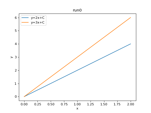
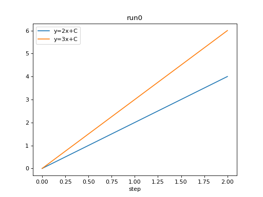
We can plot all scalar logs in a single run.
import matplotlib.pyplot as plt
from tbparse import SummaryReader
log_dir = tmpdirs['torch'].name

reader = SummaryReader(log_dir, extra_columns={'dir_name'})
df = reader.scalars
df = df[df['dir_name'] == 'run0']
df_2x = df[df['tag'] == 'y=2x+C']
df_3x = df[df['tag'] == 'y=3x+C']
plt.plot(df_2x['step'], df_2x['value'])
plt.plot(df_3x['step'], df_3x['value'])
plt.xlabel('x')
plt.ylabel('y')
plt.legend(['y=2x+C', 'y=3x+C'])
plt.title('run0')

import matplotlib.pyplot as plt
from tbparse import SummaryReader
log_dir = tmpdirs['torch'].name

reader = SummaryReader(log_dir, pivot=True, extra_columns={'dir_name'})
df = reader.scalars
df = df[df['dir_name'] == 'run0']
plt.plot(df['step'], df['y=2x+C'])
plt.plot(df['step'], df['y=3x+C'])
plt.xlabel('x')
plt.ylabel('y')
plt.legend(['y=2x+C', 'y=3x+C'])
plt.title('run0')

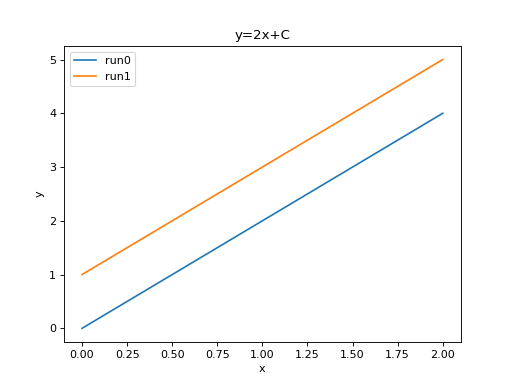
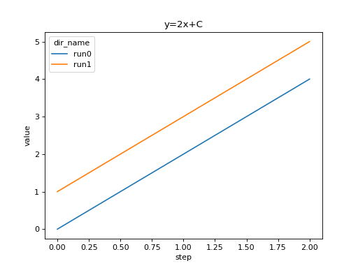
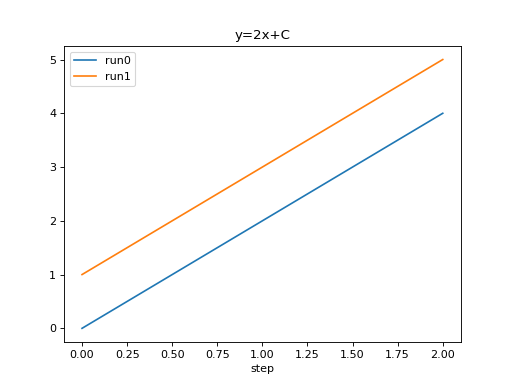
We can compare scalars across runs.
import matplotlib.pyplot as plt
from tbparse import SummaryReader
log_dir = tmpdirs['torch'].name

reader = SummaryReader(log_dir, extra_columns={'dir_name'})
df = reader.scalars
df= df[df['tag'] == 'y=2x+C']
run0 = df[df['dir_name'] == 'run0']
run1 = df[df['dir_name'] == 'run1']
plt.plot(run0['step'], run0['value'])
plt.plot(run1['step'], run1['value'])
plt.xlabel('x')
plt.ylabel('y')
plt.legend(['run0', 'run1'])
plt.title('y=2x+C')

import matplotlib.pyplot as plt
from tbparse import SummaryReader
log_dir = tmpdirs['torch'].name

reader = SummaryReader(log_dir, pivot=True, extra_columns={'dir_name'})
df = reader.scalars
run0 = df[df['dir_name'] == 'run0']
run1 = df[df['dir_name'] == 'run1']
plt.plot(run0['step'], run0['y=2x+C'])
plt.plot(run1['step'], run1['y=2x+C'])
plt.xlabel('x')
plt.ylabel('y')
plt.legend(['run0', 'run1'])
plt.title('y=2x+C')

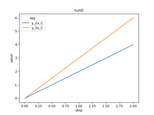
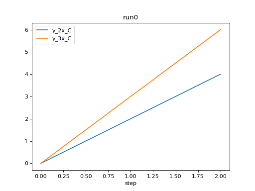
We can plot all scalar logs in a single run.
import matplotlib.pyplot as plt
from tbparse import SummaryReader
log_dir = tmpdirs['tensorboardX'].name

reader = SummaryReader(log_dir, extra_columns={'dir_name'})
df = reader.scalars
df = df[df['dir_name'] == 'run0']
df_2x = df[df['tag'] == 'y_2x_C']
df_3x = df[df['tag'] == 'y_3x_C']
plt.plot(df_2x['step'], df_2x['value'])
plt.plot(df_3x['step'], df_3x['value'])
plt.xlabel('x')
plt.ylabel('y')
plt.legend(['y=2x+C', 'y=3x+C'])
plt.title('run0')
import matplotlib.pyplot as plt
from tbparse import SummaryReader
log_dir = tmpdirs['tensorboardX'].name

reader = SummaryReader(log_dir, pivot=True, extra_columns={'dir_name'})
df = reader.scalars
df = df[df['dir_name'] == 'run0']
plt.plot(df['step'], df['y_2x_C'])
plt.plot(df['step'], df['y_3x_C'])
plt.xlabel('x')
plt.ylabel('y')
plt.legend(['y=2x+C', 'y=3x+C'])
plt.title('run0')

We can compare scalars across runs.
import matplotlib.pyplot as plt
from tbparse import SummaryReader
log_dir = tmpdirs['tensorboardX'].name

reader = SummaryReader(log_dir, extra_columns={'dir_name'})
df = reader.scalars
df= df[df['tag'] == 'y_2x_C']
run0 = df[df['dir_name'] == 'run0']
run1 = df[df['dir_name'] == 'run1']
plt.plot(run0['step'], run0['value'])
plt.plot(run1['step'], run1['value'])
plt.xlabel('x')
plt.ylabel('y')
plt.legend(['run0', 'run1'])
plt.title('y=2x+C')
import matplotlib.pyplot as plt
from tbparse import SummaryReader
log_dir = tmpdirs['tensorboardX'].name

reader = SummaryReader(log_dir, pivot=True, extra_columns={'dir_name'})
df = reader.scalars
run0 = df[df['dir_name'] == 'run0']
run1 = df[df['dir_name'] == 'run1']
plt.plot(run0['step'], run0['y_2x_C'])
plt.plot(run1['step'], run1['y_2x_C'])
plt.xlabel('x')
plt.ylabel('y')
plt.legend(['run0', 'run1'])
plt.title('y=2x+C')

Matplotlib prefers wide format in general.
Plotting with seaborn
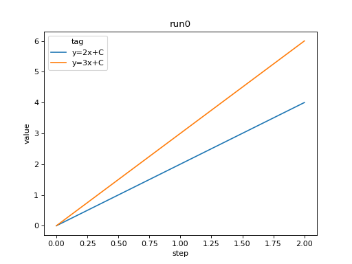
We can plot all scalar logs in a single run.
import seaborn as sns
from tbparse import SummaryReader
log_dir = tmpdirs['torch'].name

reader = SummaryReader(log_dir, extra_columns={'dir_name'})
df = reader.scalars
df = df[df['dir_name'] == 'run0']
g = sns.lineplot(data=df, x='step', y='value', hue='tag')
g.set(title='run0')
import seaborn as sns
from tbparse import SummaryReader
log_dir = tmpdirs['torch'].name

reader = SummaryReader(log_dir, pivot=True, extra_columns={'dir_name'})
df = reader.scalars
df = df[df['dir_name'] == 'run0']
g = sns.lineplot(data=df, x='step', y='y=2x+C')
g = sns.lineplot(data=df, x='step', y='y=3x+C')
g.legend(['y=2x+C', 'y=3x+C'])
g.set(ylabel='value', title='run0')
We can compare scalars across runs.
import seaborn as sns
from tbparse import SummaryReader
log_dir = tmpdirs['torch'].name

reader = SummaryReader(log_dir, extra_columns={'dir_name'})
df = reader.scalars
df = df[df['tag'] == 'y=2x+C']
g = sns.lineplot(data=df, x='step', y='value', hue='dir_name')
g.set(title='y=2x+C')

import seaborn as sns
from tbparse import SummaryReader
log_dir = tmpdirs['torch'].name

reader = SummaryReader(log_dir, pivot=True, extra_columns={'dir_name'})
df = reader.scalars
g = sns.lineplot(data=df, x='step', y='y=2x+C', hue='dir_name')
g.set(ylabel='value', title='y=2x+C')

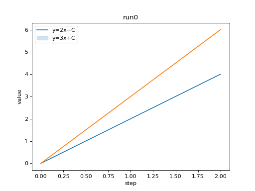
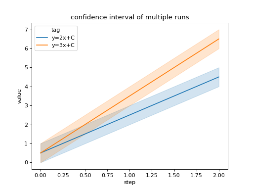
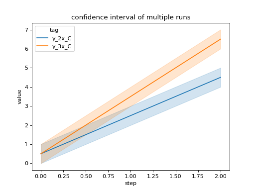
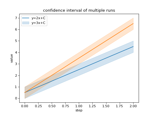
We can compare all scalar logs across runs with shaded confidence interval.
import seaborn as sns
from tbparse import SummaryReader
log_dir = tmpdirs['torch'].name

reader = SummaryReader(log_dir, extra_columns={'dir_name'})
df = reader.scalars
g = sns.lineplot(data=df, x='step', y='value', hue='tag')
g.set(title='confidence interval of multiple runs')
import seaborn as sns
from tbparse import SummaryReader
log_dir = tmpdirs['torch'].name

reader = SummaryReader(log_dir, pivot=True, extra_columns={'dir_name'})
df = reader.scalars
g = sns.lineplot(data=df, x='step', y='y=2x+C')
g = sns.lineplot(data=df, x='step', y='y=3x+C')
g.legend(['y=2x+C', 'y=3x+C'])
g.set(ylabel='value', title='confidence interval of multiple runs')

We can plot all scalar logs in a single run.
import seaborn as sns
from tbparse import SummaryReader
log_dir = tmpdirs['tensorboardX'].name

reader = SummaryReader(log_dir, extra_columns={'dir_name'})
df = reader.scalars
df = df[df['dir_name'] == 'run0']
g = sns.lineplot(data=df, x='step', y='value', hue='tag')
g.set(title='run0')
import seaborn as sns
from tbparse import SummaryReader
log_dir = tmpdirs['tensorboardX'].name

reader = SummaryReader(log_dir, pivot=True, extra_columns={'dir_name'})
df = reader.scalars
df = df[df['dir_name'] == 'run0']
g = sns.lineplot(data=df, x='step', y='y_2x_C')
g = sns.lineplot(data=df, x='step', y='y_3x_C')
g.legend(['y=2x+C', 'y=3x+C'])
g.set(ylabel='value', title='run0')

We can compare scalars across runs.
import seaborn as sns
from tbparse import SummaryReader
log_dir = tmpdirs['tensorboardX'].name

reader = SummaryReader(log_dir, extra_columns={'dir_name'})
df = reader.scalars
df = df[df['tag'] == 'y_2x_C']
g = sns.lineplot(data=df, x='step', y='value', hue='dir_name')
g.set(title='y=2x+C')

import seaborn as sns
from tbparse import SummaryReader
log_dir = tmpdirs['tensorboardX'].name

reader = SummaryReader(log_dir, pivot=True, extra_columns={'dir_name'})
df = reader.scalars
g = sns.lineplot(data=df, x='step', y='y_2x_C', hue='dir_name')
g.set(ylabel='value', title='y=2x+C')
We can compare all scalar logs across runs with shaded confidence interval.
import seaborn as sns
from tbparse import SummaryReader
log_dir = tmpdirs['tensorboardX'].name

reader = SummaryReader(log_dir, extra_columns={'dir_name'})
df = reader.scalars
g = sns.lineplot(data=df, x='step', y='value', hue='tag')
g.set(title='confidence interval of multiple runs')
import seaborn as sns
from tbparse import SummaryReader
log_dir = tmpdirs['tensorboardX'].name

reader = SummaryReader(log_dir, pivot=True, extra_columns={'dir_name'})
df = reader.scalars
g = sns.lineplot(data=df, x='step', y='y_2x_C')
g = sns.lineplot(data=df, x='step', y='y_3x_C')
g.legend(['y=2x+C', 'y=3x+C'])
g.set(ylabel='value', title='confidence interval of multiple runs')
Seaborn prefers long format in general.
Plotting with pandas
We can plot all scalar logs in a single run.
from tbparse import SummaryReader
log_dir = tmpdirs['torch'].name

reader = SummaryReader(log_dir, extra_columns={'dir_name'})
df = reader.scalars
df.set_index('step', inplace=True)
df = df[df['dir_name'] == 'run0']
df_2x = df[df['tag'] == 'y=2x+C']
df_3x = df[df['tag'] == 'y=3x+C']
ax = df_2x.plot.line(title='run0')
df_3x.plot.line(ax=ax)
ax.legend(['y=2x+C', 'y=3x+C'])

from tbparse import SummaryReader
log_dir = tmpdirs['torch'].name

reader = SummaryReader(log_dir, pivot=True, extra_columns={'dir_name'})
df = reader.scalars
df.set_index('step', inplace=True)
df = df[df['dir_name'] == 'run0']
df.plot.line(title='run0')
We can compare scalars across runs.
from tbparse import SummaryReader
log_dir = tmpdirs['torch'].name

reader = SummaryReader(log_dir, extra_columns={'dir_name'})
df = reader.scalars
df = df[df['tag'] == 'y=2x+C']
run0 = df.loc[df['dir_name'] == 'run0', ['step', 'value']].rename(columns={'value': 'run0'})
run1 = df.loc[df['dir_name'] == 'run1', ['step', 'value']].rename(columns={'value': 'run1'})
df = run0.merge(run1, how='outer', on='step', suffixes=(False, False))
df.set_index('step', inplace=True)
df.plot.line(title='y=2x+C')
from tbparse import SummaryReader
log_dir = tmpdirs['torch'].name

reader = SummaryReader(log_dir, pivot=True, extra_columns={'dir_name'})
df = reader.scalars
run0 = df.loc[df['dir_name'] == 'run0', ['step', 'y=2x+C']].rename(columns={'y=2x+C': 'run0'})
run1 = df.loc[df['dir_name'] == 'run1', ['step', 'y=2x+C']].rename(columns={'y=2x+C': 'run1'})
df = run0.merge(run1, how='outer', on='step', suffixes=(False, False))
df.set_index('step', inplace=True)
df.plot.line(title='y=2x+C')

We can plot all scalar logs in a single run.
from tbparse import SummaryReader
log_dir = tmpdirs['tensorboardX'].name

reader = SummaryReader(log_dir, extra_columns={'dir_name'})
df = reader.scalars
df.set_index('step', inplace=True)
df = df[df['dir_name'] == 'run0']
df_2x = df[df['tag'] == 'y_2x_C']
df_3x = df[df['tag'] == 'y_3x_C']
ax = df_2x.plot.line(title='run0')
df_3x.plot.line(ax=ax)
ax.legend(['y=2x+C', 'y=3x+C'])

from tbparse import SummaryReader
log_dir = tmpdirs['tensorboardX'].name

reader = SummaryReader(log_dir, pivot=True, extra_columns={'dir_name'})
df = reader.scalars
df.set_index('step', inplace=True)
df = df[df['dir_name'] == 'run0']
df.plot.line(title='run0')
We can compare scalars across runs.
from tbparse import SummaryReader
log_dir = tmpdirs['tensorboardX'].name

reader = SummaryReader(log_dir, extra_columns={'dir_name'})
df = reader.scalars
df = df[df['tag'] == 'y_2x_C']
run0 = df.loc[df['dir_name'] == 'run0', ['step', 'value']].rename(columns={'value': 'run0'})
run1 = df.loc[df['dir_name'] == 'run1', ['step', 'value']].rename(columns={'value': 'run1'})
df = run0.merge(run1, how='outer', on='step', suffixes=(False, False))
df.set_index('step', inplace=True)
df.plot.line(title='y=2x+C')

from tbparse import SummaryReader
log_dir = tmpdirs['tensorboardX'].name

reader = SummaryReader(log_dir, pivot=True, extra_columns={'dir_name'})
df = reader.scalars
run0 = df.loc[df['dir_name'] == 'run0', ['step', 'y_2x_C']].rename(columns={'y_2x_C': 'run0'})
run1 = df.loc[df['dir_name'] == 'run1', ['step', 'y_2x_C']].rename(columns={'y_2x_C': 'run1'})
df = run0.merge(run1, how='outer', on='step', suffixes=(False, False))
df.set_index('step', inplace=True)
df.plot.line(title='y=2x+C')

Pandas prefers wide format in general.